Link: https://www.kaggle.com/c/predict-ai-model-runtime
Problem Type: learning to rank
Input: The structure of a neural network (the nodes and edges of the graph)
- You get features for each node of the network
- You also get the model config
Output:
- The order of different model configs (i.e. you are predicting how fast each model runs, and ordering those model IDs)
- For the
tile:xlacollection, only the first 5 entries will be considered and the rest will be ignored. - For the
layout:*collections, all entries will be considered (you should output a permutation of the number of configurations!).
- For the
Eval Metric: Kendall Tau correlation AND custom metric for the top-k predictions
Summary
- The goal is to predict the runtime of an AI model based on its characteristics, such as the number of parameters/the number of layers/hardware configuration.
- you have to predict the runtime for many different types of ml models
- e.g. bert, resnet50
- you have to predict the runtime for many different types of ml models
- Glossary:
xla: accelerated linear algebra. it’s an open-source compiler for machine learning: https://www.tensorflow.org/xlaHlo: high level optimizer
Important notebooks/discussions
- understanding the competition
- explaining tensor tile, tensor shard, simulated annealing, and langevin dynamics
- video links to googlers explaining mroe about the problem, and considerations
Solutions
-
(1st) Speed up iteration time. Custom attention layer to compare configs throughout the network
- https://www.kaggle.com/competitions/predict-ai-model-runtime/discussion/456343
- solution code: https://github.com/thanhhau097/google_fast_or_slow/tree/main
- We pruned and compressed the layout graphs in order to increase the efficiency of our experiments speedup iteration
- They noticed that only
Convolution,DotandReshapewere configurable nodes - So their pruning strat was: for each graph, only keep the nodes that were either configurable models themselves or were connected to a configurable node
- this reduced vram usage by 4x and increased training speed by 5x
- They noticed that only
- deduplication: they found that configs for different network layouts had many duplications
- and “the runtime for the duplicated configs can vary quite a bit and make training less stable”
- why would the runtime be different if they were the same?
- probably because of page faults? or leaky memory in their computer?
- or maybe on subsequent runs, they were cached
- I guess the first run would be the most accurate (since it’s fresh)
- probably because of page faults? or leaky memory in their computer?
- loading all the data still used lots of ram
- so they compressed node_config_feat and only decompressed it on-the-fly in the dataloader data compression
- they realized that each of the 6 columns in node_config_feat only has 7 possible values
- so each row can be represented as a base 7 integer: from 0 to 7
- they stored the compressed data as a numpy array
- https://github.com/thanhhau097/google_fast_or_slow/blob/main/data/data_compression.py
- code
def vec_to_int(vec: np.ndarray) -> np.ndarray:
    # Powers of 7: [1, 7, 49, 343, 2401, 16807]
    powers_of_7 = np.array([7**i for i in range(6)])
    return np.dot(vec, powers_of_7).astype(np.int32)
- they realized that each of the 6 columns in node_config_feat only has 7 possible values
- by loading all data to memory at the beginning of training, they reduced IO/CPU bottlenecks considerably and allowed them to train faster. speedup iteration
- change pad value in
node_featfrom 0 to -1- they realized that values in
node_config_featwas -1 padded, but values innode_featwas 0-padded- this was a problem cause for some features 0 is a valid value
- so they changed
node_featto be -1 padded so that they can use a single embedding matrix for bothnode_feat[134:]andnode_config_featplaceholder for invalid values
- they realized that values in
- normalize features
- They used
StandardScalerfor these features:node_feat[:134]- cause some features were
*_sumand*_product, which can have high values - these disrupt the optimization
- cause some features were
- They used
- network architecture
- for the graph convolutional layer itself:
- SAGEConv was good
- GAT variants didn’t work (Graph attention)
- but self-channel attention and cross-config attention was good
- SAGEConv was good
- Squeeze-and-Excitation layer
- crossConfigAttention
- Another dimension that we can exploit attention is the batch plane (cross-configs). We designed a very simple block that allows the model to explicitly “compare” each config against the others throughout the network. We found this to be much better than letting the model infer for each config individually and only compare them implicitly via the loss function (
PairwiseHingeLoss). The attention code is as follows:- code
class CrossConfigAttention(nn.Module):
    def __init__(self):
        super().__init__()
        self.temperature = nn.Parameter(torch.tensor(0.5))

    def forward(self, x):
        # x of shape (nb_configs, nb_nodes, nb_features)
        scores = (x / self.temperature).softmax(dim=0)
        x = x * scores
        return x
- code
- By applying this simple layer after the self-channel attention at every block of the network, it gave us a huge boost for default collections.
- it’s applied like so:
- Note: the output of the forward layer is (nb_configs, nb_nodes, nb_features) since multiplication and sigmoid are scalar operations
- cause dim=0 means: This operation will get probabilities that sum up to 1 across the dimension 0
- I’m not sure why they concat the cross attention with the self channel attention. I don’t think they need to do that?
- oh it’s answered: (we concat the output with its input to preserve the individuality of each sample)
- note that they do:
scores = (x / self.temperature)- but I think that scores = (x * self.temperature) works as well since self.temperature is used once.
- Another dimension that we can exploit attention is the batch plane (cross-configs). We designed a very simple block that allows the model to explicitly “compare” each config against the others throughout the network. We found this to be much better than letting the model infer for each config individually and only compare them implicitly via the loss function (
- for the graph convolutional layer itself:
- However, since the prediction depends on the batch, we can leverage it further by applying TTA (Test Time Augmentation) to generate
N(10) permutations of the configs and average the result after sorting it back to the original order.- I think the author is saying: inferencing is unstable. So to get better answers, we generate 10 permutations of the same config, then average the result, so the inferred value is smoohter.
- but I don’t get it. ppl usually say this when ensembling, not “in a layer”. also why does he mention batch size during inference?
- https://github.com/thanhhau097/google_fast_or_slow/blob/626c463dfb02abd739616773ca74f34e38635c71/dataset.py#L441
- I think he just means that he’s enssembling the results 10 times
- he does: # shuffle runtime and config feats
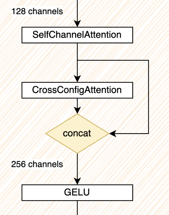
- To create our Linear/Conv blocks we followed the good practices in computer vision. We start by using
InstanceNormto normalise the input feature map, followed byLinear/SAGEConv layer,SelfChannelAttetionandCrossConfigAttetion(we concat the output with its input to preserve the individuality of each sample). Then, we sum the residual connection and finish with Gaussian Error Linear Unit (GELU) and dropout. PairwiseHingeLoss
- https://www.kaggle.com/competitions/predict-ai-model-runtime/discussion/456343
-
(2nd) Invented their own DiffMat Loss
- https://www.kaggle.com/competitions/predict-ai-model-runtime/discussion/456365
- solution code: https://github.com/Obs01ete/kaggle_latenciaga/tree/master
- data cleaning
- like (1st), they found duplicated configs (with diff runtimes). so they deduped them, and keept the config that had the lowest runtime
- didn’t use unet graphs cause
unet_3d.4x4.bf16was badly corrupted - they repackaged each NPZ so that each config+runtime measurement could be loaded without needing to load the entire NPZ
- model
- All GNN layers are SageConv layers with residual connections whenever the number of input and output channels are the same.
- Features produced by the GNN layer stack are transformed to one value per node and then sum-reduced to form a single graph-wise prediction.
- not sure what sum-reduced means. but probably mean?
- training
- Models trained with a ranking loss (ListMLE Loss, marginRankingLoss) heavily outperformed element-wise losses (MAPE, etc).
- “The batch is organized into 2 levels of hierarchy: the upper level is different graphs, and the lower level is the same graph and different configurations, grouped in microbatches of the same size (also known as slates)”
- todo: understand
- hyperparams
- Adam/AdamW optimizer,
- Learning rate 1e-3,
- 400k iterations,
- Step learning rate scheduler at 240k, 280k, 320k, and 360k by factor of
1/sqrt(10).
- Losses used for training:
- ListMLE Loss for Layout-NLP,
- A novel DiffMat loss for Tile,
- For Layout-XLA, it is a combination of 2 losses: the DiffMat loss and MAPE loss.
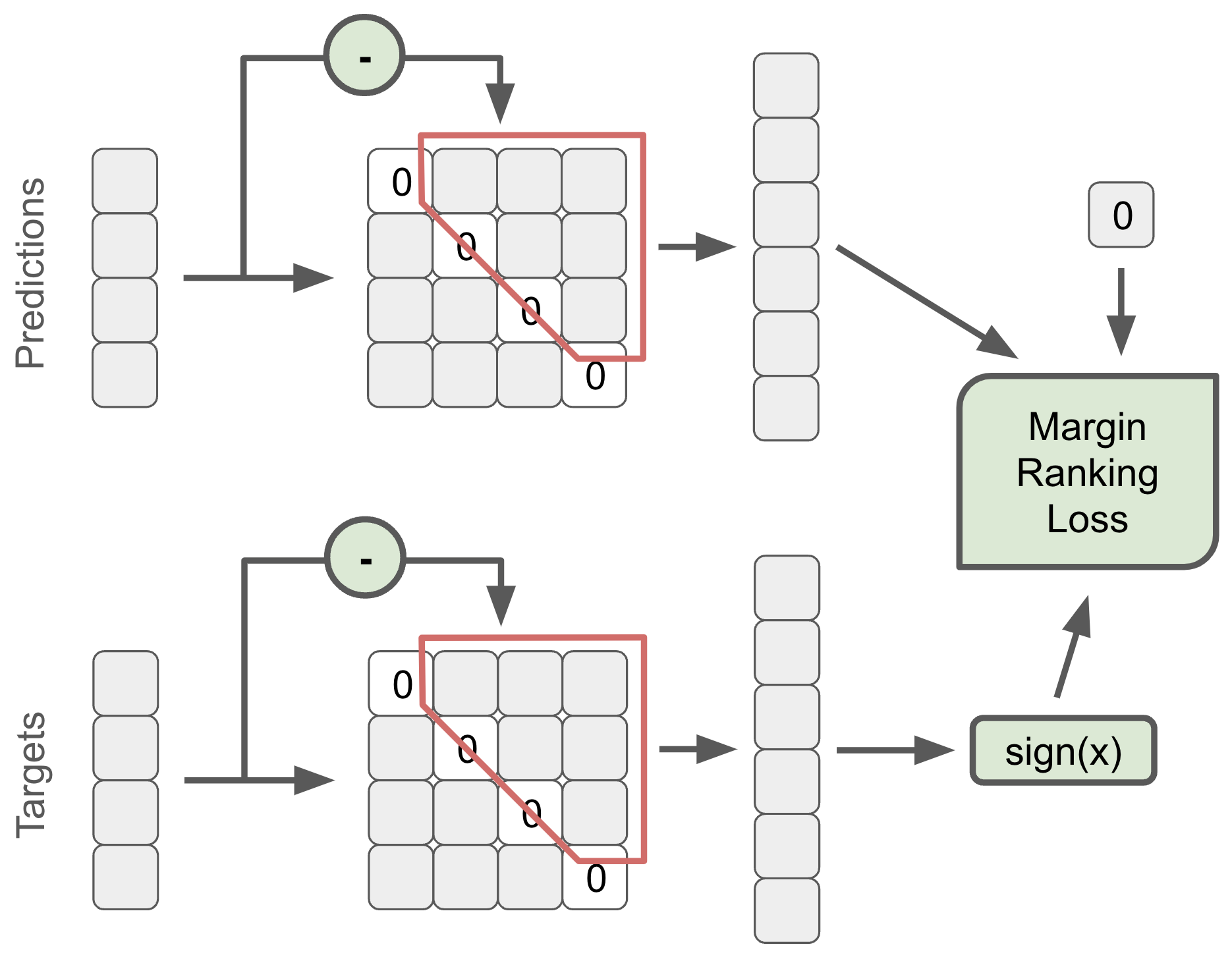
- DiffMat Loss custom loss
- The idea is to use the difference matrix between …
- the difference matrix reminds me of marginRankingLoss (since it’s euclidian distance)
- this is fed into marginRankingLoss
- I’m not sure what “Margin Ranking Loss with a margin of 0.01 is applied between predicted values and zeros” means
- this diagram is kinda vague:
- I tried reading their code but couldn’t find it.
- this diagram is kinda vague:
- The idea is to use the difference matrix between …
- data recovery
- We tried to find the damaged data and remove it in an automatic manner by computing block-wise entropy of the runtimes between adjacent blocks.
- what didn’t work:
- Online hard negative mining “since train loss is nowhere near zero,”
- I think this is because the model already isn’t learning positive OR negative examples well
- The model needs to first learn well from the “easier” examples before introducing “harder” ones.
- Train 4 folds and merge by mean latency and by mean reciprocal rank (MRR)
- Online hard negative mining “since train loss is nowhere near zero,”
-
(3rd) Novel feature generation
-
(4th) Only uses a multi layer perceptron - very clever feature engineering
- https://www.kaggle.com/competitions/predict-ai-model-runtime/discussion/456462
- features:
- a few of the features were just the original columns (but untransformed): node_feat_index
-
(5th) - Transformer to compress dimensions rather than flattening
- https://www.kaggle.com/competitions/predict-ai-model-runtime/discussion/456093
- solution code: https://github.com/knshnb/kaggle-tpu-graph-5th-place
- Preprocessing
- Transformer to compress dimensions rather than flattening
- each node in the graph contained 6 dimensions.
- each dimension has 30 features.
- before feeding this into the neural net, he could’ve flattened this 2D array of features into a 1D array (of length: 30 * 6)
- HOWEVER, this removes information that says: “these 30 features were from the same dimension”
- the model needs to implicitly learn this
- So to compress it, he used a transformer to transform the (6, 30) input into a (6, 15) output vector
- Note: he treats each of the dimensions as a token when feeding it to the transformer
- finally, he took the sum in the token dimension to reduce it to a vector of length (15)
- this was the key part.
- each node in the graph contained 6 dimensions.
- Transformer to compress dimensions rather than flattening
- Tips
- use the same opcode embedding for unary operations such as abs, ceil, cosine, etc.
- override layout_minor_to_major by layout config features for configurable nodes
- DropEdge
- training only
- apply log transformation to input features
- oversampling
- load layout config data by numpy’s mmap mode to save RAM
- This is one of their graphConv layers
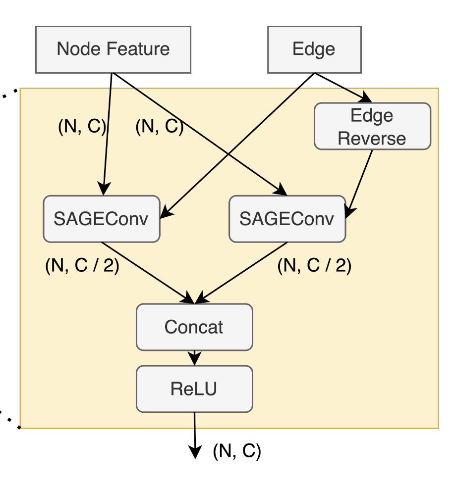
- notice how they had a function to reverse the edge before feeding it into another sageConv
- code
	self.gconv = SAGEConv(mid_ch, mid_ch // 2, ...)
	self.rev_gconv =SAGEConv(mid_ch, mid_ch // 2, ...)

	rev_edge_index = torch.flip(edge_index, (0,))
	x = torch.cat([self.gconv(x, edge_index), self.rev_gconv(x, rev_edge_index)], dim=-1))
	```
- What Didn’t Work
- graph pooling
- pretrain on the tile dataset and finetune on the layout dataset
- graph normalization
- dropout node
- GAT, GATv2, GIN
- GATV2 DID NOT WORK???!?!??!
- fp16
- pseudo label
-
(6th) - graph isomorphism network Graph Attention Networks (GATs)
- solution code: https://github.com/hengck23/solution-predict-ai-model-runtime
- learn on subsets
- main problem:
- we have very large graph as input. how to design learning model and algorithm that can fit into gpu memory?
- solution
- instead of using the whole graph, we can reduce it by considering only the 5-hop neighbours from node marked as “config id”. We call this 5-hop-neighbour subgraph. We think this is reasonable becuase since we are comparing relative ranking of 2 graphs, and we just need to input the “difference nodes” (instead of the whole graph) to the neural net.
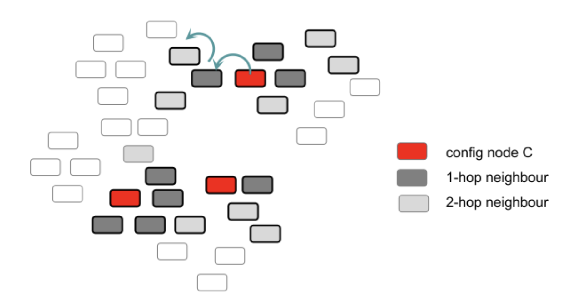
- main problem:
- used gradient accumulation
- normalization is important
- it works well with gradient accumulation
- they used “graph instance norm” over the nodes
- GraphNorm: A Principled Approach to Accelerating Graph Neural Network Training https://arxiv.org/abs/2009.03294
- they used a custom type of pairwise ranking loss. custom loss
- I don’t understand it, but it’s not hard, and here’s the code: https://github.com/hengck23/solution-predict-ai-model-runtime/blob/998d74a026a7b82705c458b81e67db8db5c8370b/src/res-gin4-pair-hop5-layout/myloss.py#L59
- We try both SAGE-conv[2] and GAT-conv[4]. GAT-conv gives better results.
- Since we are interested in top 5 ranks, we find ListMLE Loss is a better loss.
Takeaways
- find ways to reduce your input dataset as much as possible
- use data compression if you need to. This speeds up your iteration time by a lot
- do not train on padded columns if you don’t need to
- Graph Attention Networks (GATs) work well.
- people ran into smoothing problems, and used techniques like DropEdge and
- ListMLE Loss is a decent loss
- but there’s lots of opportunities here to make your own loss (and do well)
- people’s models weren’t very deep. A few SAGEConv or even multi layer perceptron works well