Link: https://www.kaggle.com/c/LANL-Earthquake-Prediction
Problem Type: regression, signal processing
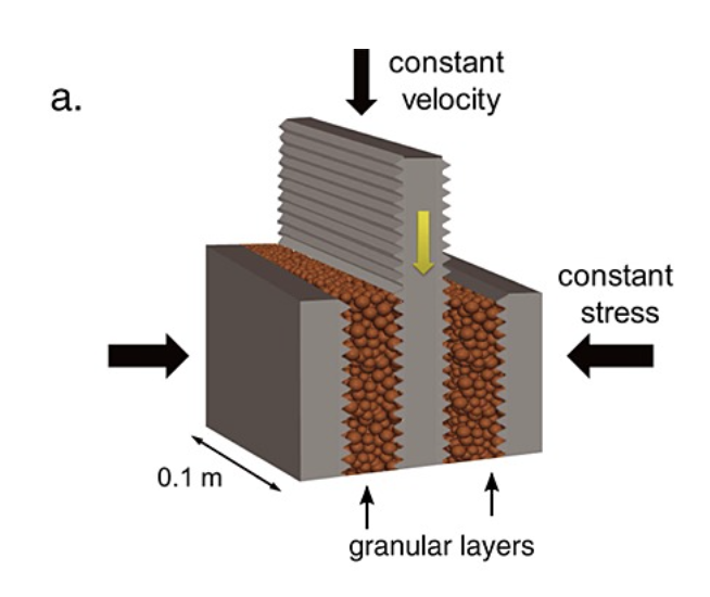
Input: the acoustic data (the shaky line that is draw by seismometers)
Output: the time (in seconds) until the next laboratory earthquake
- “We define large failure events as times for which stress drop exceeds 0.05 MPa within 1 ms.”
Eval Metric: Mean absolute error (MAE)
Summary
- This was a competition with a high leaderboard shakeup because ppl overfit the public LB
- Your goal is to predict the time remaining before laboratory earthquakes occur from real-time seismic data.
- these aren’t real earthquakes. it’s a lab setup:
- Why did many ppl overfit the public lb?
- they blindly subtracted the data by the mean (of the acoustic data) during training, but the mean shifts in the test set
Important notebooks/discussions
Solutions
-
(1st) Add noise to denoise median statistic PSI’s solution
- https://www.kaggle.com/competitions/LANL-Earthquake-Prediction/discussion/94390
- solution code:
- “After doing abovementioned signal manipulation, we had more trust in our calculated features and could focus on better studying differences between train and test data feature distributions”
- we calculated a handful of features for train and test and tried to find a good subset of full earth-quakes in train, so that the overall feature distributions are similar to those of the full test data.
- a simple shuffled 3-kfold
- adversarial validation shows that the signal had a certain time-trend that made mean or quantile features unreliable
- e.g. mean number of “spikes” in a sliding window of 100ms of data
- One of our best final LGB model only used four features:
- (i) number of peaks of at least support 2 on the denoised signal
- 0.67 Pearson’s Correlation Coefficient seems about right for the “number of peaks” feature.
- (ii) 20% percentile on std of rolling window of size 50
- (iii and iv) 4th and 18th coefficient in the series of Mel frequency cepstral coefficients (MFCC)
- (i) number of peaks of at least support 2 on the denoised signal
- Those 4 are decently uncorrelated between themselves, and add good diversity.
- For each feature we always only considered it if it has a p-value >0.05 on a KS statistic of train vs test. considering features
- why does adding noise then subtracting the median de-noise the signal? Add noise to denoise median statistic
- https://www.kaggle.com/competitions/LANL-Earthquake-Prediction/discussion/94390#553415
- If you take mean of train and test, you can see the testing set has a higher mean than the training set. Therefore we elect to subtract the mean to make the test more similar to the train. However, even after subtracting the mean, the feature related to median (e.g.
np.median(z)) still had dissimilarities between the train and test segment. To solve this, we tried subtracting solely the median (instead of the mean), but this still did not solve the issue. Therefore we injected small amount of noise, and then subtracted the median.- After adding the “noise” (std 0.5), which is actually lower or in the range of the expected accuracy of the sensor (1),
absmedianbehaves very normally (same distribution for train and test)- where
z = z - np.mean(z); absmedian = np.median(abs(z)) - I think because after noise was injected, the median they subtract by is the TRUE median (much less disturbed by random points)
- “with the raw data, the median for the earthquakes were: 3, 4, 4,5, or 5” - by CPMP
- Once noise is added then median value distribution is not as sparse.
- where
- After adding the “noise” (std 0.5), which is actually lower or in the range of the expected accuracy of the sensor (1),
- why did they want to subtract by median not mean?
- cause
medianis more robust to outliers thanmean
- cause
- Our features are then calculated on this manipulated signal.
- KS statistic showed that there’s a drift between the train and test data
- so we decided to sample the train data to make it look more like we expect test data to look like (only from looking at feature distributions)
- we calculated a handful of features for train and test and tried to find a good subset of full earth-quakes in train, so that the overall feature distributions are similar to those of the full test data.
- We did this by sampling 10 full earthquakes multiple times (up to 10k times) on train, and comparing the average KS statistic of all selected features on the sampled earthquakes to the feature dists in full test.
- what does sampling 10 full earthquakes multiple times mean?
- https://www.kaggle.com/competitions/LANL-Earthquake-Prediction/discussion/94390#544281
- In training data we have 17 earthquakes. We sampled 10_000 times 10 earthquakes out of that
- i.e. 10,000 from 17 choose 10
- In training data we have 17 earthquakes. We sampled 10_000 times 10 earthquakes out of that
- https://www.kaggle.com/competitions/LANL-Earthquake-Prediction/discussion/94390#550006
- Each dot in that picture: (1) sample a certain number of earthquakes from train, (2) calculate KS statistic for each feature between sampled train and full test, (3) draw KS value on plot. Best sampling is based on lowest average KS statistic across features.
- they used
scipy.stats.ks_2samp(train, test)
- https://www.kaggle.com/competitions/LANL-Earthquake-Prediction/discussion/94390#544281
- what does sampling 10 full earthquakes multiple times mean?
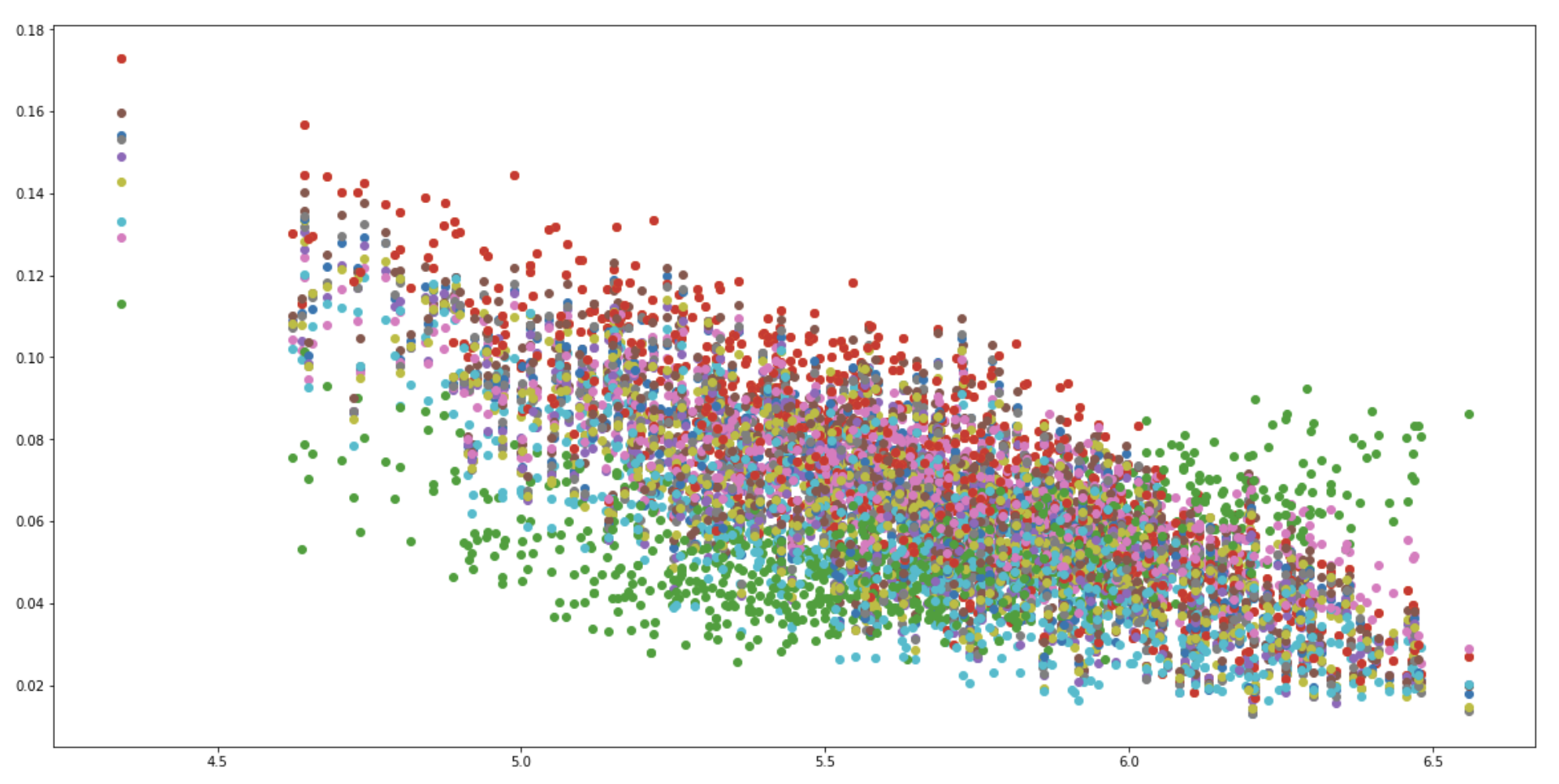
- “The x-axis is the average target of the selected EQs in train and the y-axis is the KS statistic on a bunch of features comparing the distribution of that feature for the selected EQs vs the full test data. We can see that the best average KS-statistic is somewhere in the range of 6.2-6.5. You can also see nicely here that a problematic feature like the green one deviates clearly from the rest, this would be a feature we would not select in the end.”
- time since an event occurred as an auxiliary target: “We have one additional binary logloss with the target specifying if the time to failure (ttf) is <0.5 and one further MAE loss on the target of time-since-failure.”
- Neural nets trained on raw data failed
- so didn’t consider using denoise autoencoder
-
(2nd) lots of signal processing features. made train data look like test data
- https://www.kaggle.com/competitions/LANL-Earthquake-Prediction/discussion/94369
- made train data look like test data (the img from https://www.kaggle.com/c/LANL-Earthquake-Prediction/discussion/90664#latest-535844)
- features:
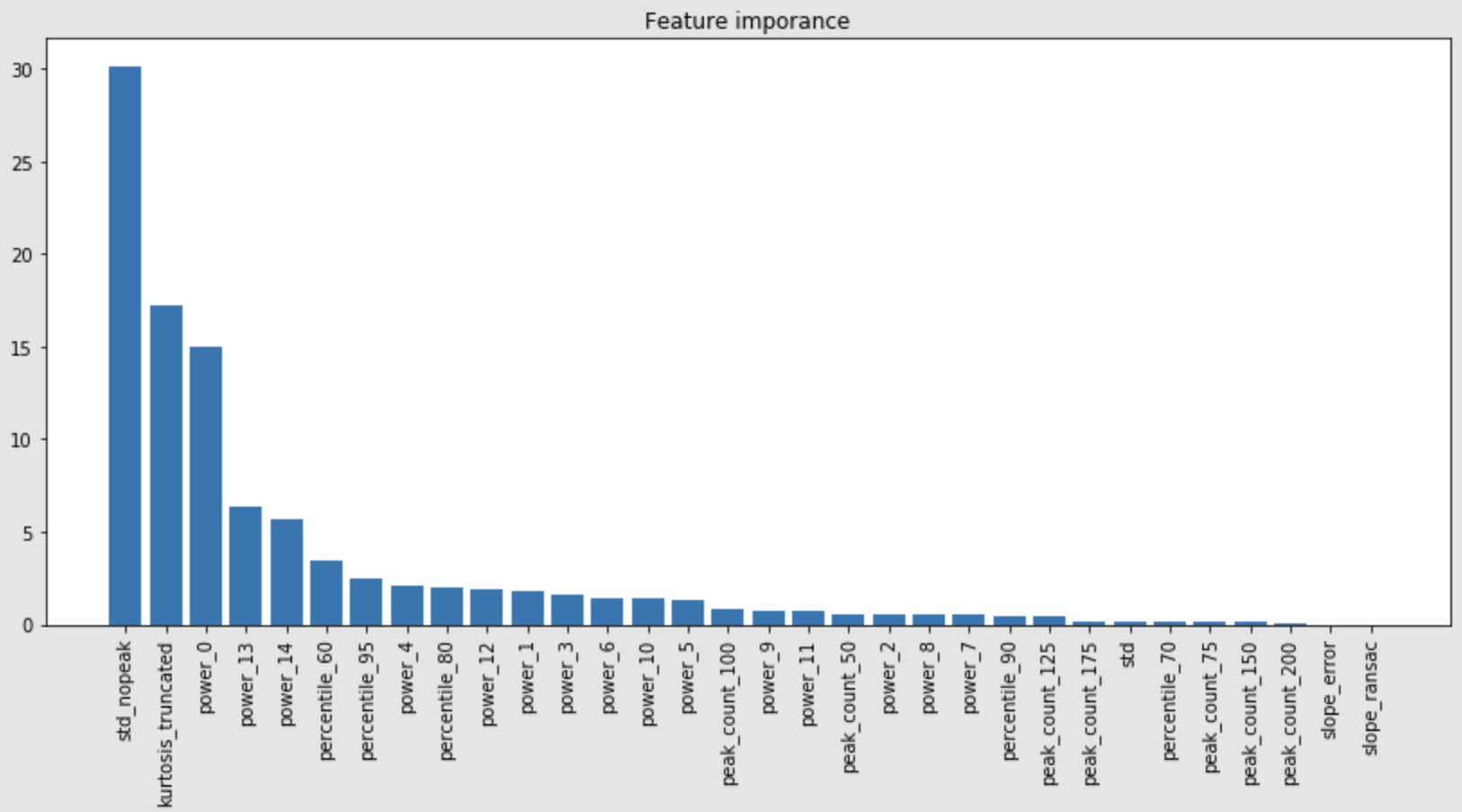
- they listed many features. interesting ones were:
- std_nopeak: Std of data that are not part of peaks
- kurtosis_truncated: Kurtosis of data with abs(v - mean(v)) < 20
- trend: slope of robust linear regression to 30 sub chunks of std_truncated
- trend_error: Abs difference in the slope of RANSAC and HuberRegressor
- power spectrum: Fast-Fourier Transform the data and average the absolute value in 15 bins
- used subtraction to avoid dependence on mean:
- 95 percentile - 5 percentile
- peak height is defined as: (max - min)/2.
- The std_truncated (std instead of kurtosis in kurtosis_truncated) works almost as well as std_nopeak.
- feature importance
- they listed many features. interesting ones were:
- I THINK THEY DIDN’T HAVE CV. THEY JUST USED INTUITION
- “I felt there aren’t much information we can extract from the acustic data and I felt I have more than enough features to get all the information”
- used a Default parameter CatBoost single model
-
(3rd) made train data look like test data LSTM
- https://www.kaggle.com/competitions/LANL-Earthquake-Prediction/discussion/94459
- Already mentioned in the discussion , we expected test from p4677.
- the yhat is found via (NOTE: I don’t completely understand this) :
best_y = np.median(np.hstack([np.repeat(cycle_len, int(100*cycle_len)) for cycle_len in chunk_length_list]))- the code creates a long array by repeating each chunk length value proportionally to the length itself.
- Then it calculates the median of that array.
- The assumption behind the code is likely that the chunk lengths that occur most often are more “typical” or “representative” and thus are the “best” values
-
cycle_len in chunk_length_list: This iterates over eachcycle_lenin a given list of chunk lengths, referred to aschunk_length_list.
-
np.repeat(cycle_len, int(100*cycle_len)): For eachcycle_lenfrom thechunk_length_list, it repeatscycle_lenint(100*cycle_len)times. For example, ifcycle_lenis 2, it creates an array[2, 2, 2,...]with lengthint(100*2) = 200.
-
np.hstack([]): This function is used for horizontally stacking all the arrays created for eachcycle_leninchunk_length_listand making one single flattened array.
-
np.median(): Finally, the median of the created array is calculated and is stored inbest_y.
- the code creates a long array by repeating each chunk length value proportionally to the length itself.
-
(7th) Used Signal processing techniques to generate features
- https://www.kaggle.com/competitions/LANL-Earthquake-Prediction/discussion/94359
- one EarthQuake (EQ) out CV
- Calculated around 200 features based mainly on Short-time Fourier Transform (STFT)
Takeaways
- (1st and 2nd) made a sub-train set that is the same distribution of test. if you can figure out how the test distribution would look like
- Sometimes models will still generalize better if you give them diverser training examples and aligning training and test sets can be really overfitty
- You always have to pay attention to the mean / median of your test/train dataset. These tricks can help:
- time since an event occurred as an auxiliary target